Edit, predict, evaluate your proteins structures in bulk with LiteFold

We just launched something new at LiteFold, a structure prediction editor. Yes, an editor, not just a prediction tool. Let me explain.
After AlphaFold 2 and 3 came out of DeepMind, the open-source community didn’t sit back. They’ve been actively building strong alternatives, not just replicas, but next-gen structure predictors. Some of the standout ones include OpenFold from AQ Laboratory, ProteinX by ByteDance, Chai-1/2 by Chai Discovery, and Boltz 1/2 by MIT. What makes these exciting is that they're not just doing plain protein folding anymore they’re moving towards generalized biomolecular structure prediction. That includes antibody complexes, protein-RNA structures, ligands the whole range. If you're skeptical or wondering how Boltz-2 stacks up against AlphaFold, take a close look at the latest benchmarks. The results speak for themselves.
| Metric | AlphaFold 2 | AlphaFold 3 | Boltz-2 |
|---|---|---|---|
| Antibody–Antigen DockQ > 0.23 | 27% (AF2-Multimer v2.3) | 85% | 53% |
| Protein–Protein DockQ > 0.23 | ~60% | 83% | ~67% |
| Protein–Ligand Pose Accuracy (<2Å) | Not supported | ~66% (PoseBusters) | 62.5% (FEP+ subset) |
| Protein–RNA LDDT | ~60 | 78 | 74 |
| RMSF Pearson (ATLAS) | – | – | 0.82 |
| RMSF Spearman (mdCATH) | – | – | 0.77 |
| Binding Affinity Pearson (FEP+) | – | – | 0.62–0.66 |
| Binding Affinity R² (FEP+) | – | – | ~0.55 |
| SKEMPI-2 ΔΔG Pearson | – | 0.86 | – |
| Structure-only Inference Time | ~30–90 min | ~5–20 min | ~5–15 sec |
| Binding Affinity Inference Time | Not supported | Not supported | ~5–15 sec |
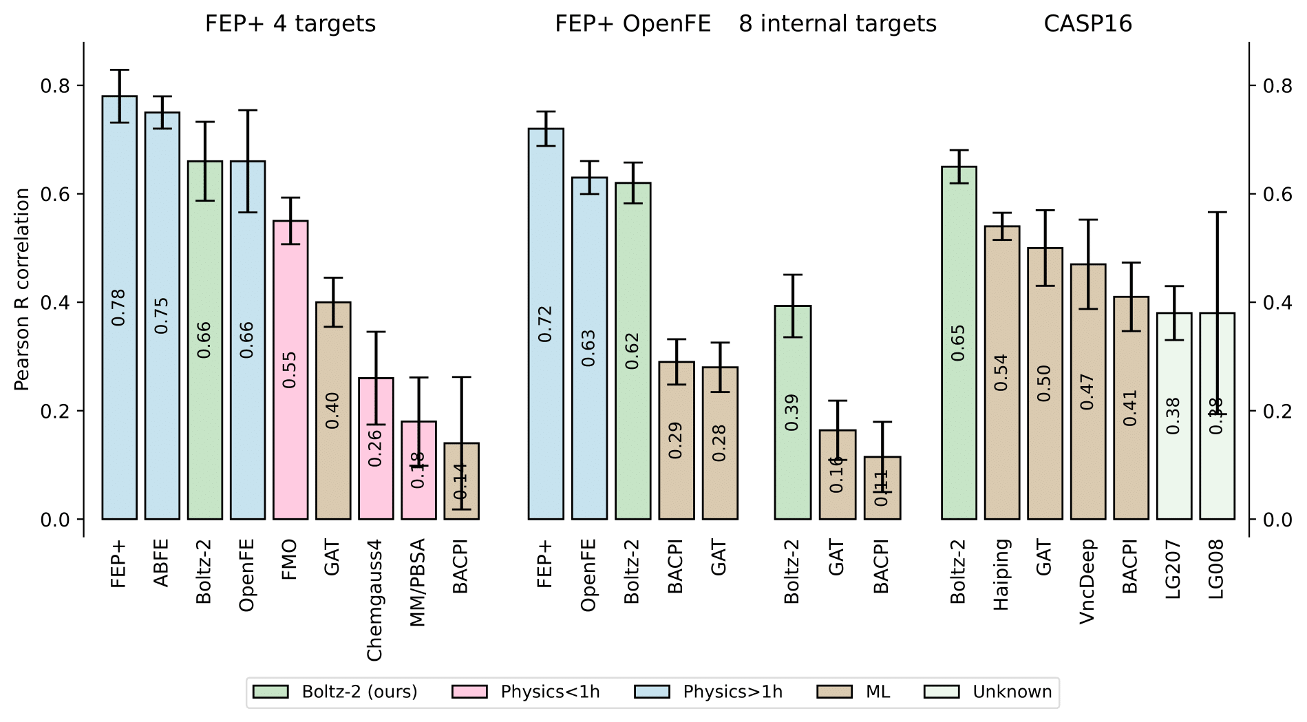
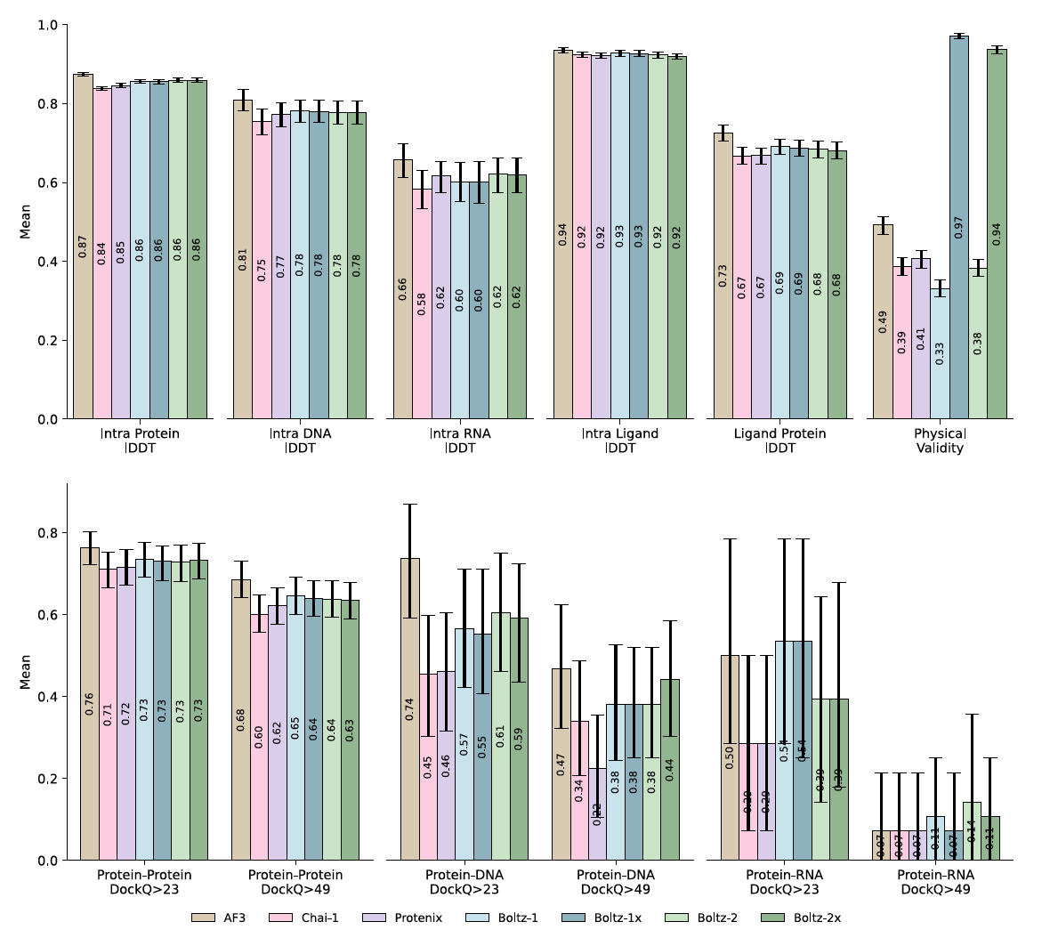
From the above table, you can see that Boltz-2 performs competitively with AlphaFold 3 across several benchmarks and outperforms it in inference speed and flexibility. For instance below images shows the comparisons between Boltz-2 model and others in CASP-16 and other affinity related benchmarks.
While AlphaFold 3 is not technically Open Source, Boltz-2 brings a lot of that capability in an open, fast, and extendible way. That’s why we chose it. We’re excited to share that LiteFold’s structure prediction editor is powered by Boltz-2 under the hood.
We are on a mission to make molecular and structural biology related experiments easier than ever. Whether you are doing research on protein design, drug design or want to run and organize your experiments, LiteFold helps to manage that with ease. Try out, it's free.
What's this Structure Prediction Editor?
The most common input for structure prediction is still FASTA files. You can define multiple chains: proteins, DNA/RNA, small molecules (via SMILES or CCD codes) and even point to precomputed MSAs. For most basic use cases, that’s enough. But if you're using the Boltz‑2 model, you're leaving a lot of power on the table by sticking to FASTA. Here's what you can not do in FASTA:
- No Modified Residues: You can’t specify non-standard amino acids or modified nucleotides. This means you’re limited to plain sequences, which doesn’t reflect real biological scenarios where modifications are common (e.g., phosphoserine, methylated cytosine).
- No Covalent Bonds: You can’t define explicit bonds between atoms, for example, a covalent link between a ligand and a residue. That’s essential if you’re modeling inhibitors or covalently bound cofactors.
- No Pocket Constraints: You can’t specify where a ligand should bind, e.g., “this SMILES should interact with residues 35, 89, and 110 in chain A.” Boltz allows adding physical constraints to guide sampling around pockets. FASTA can’t capture this.
- No Affinity Prediction Setup: You can’t flag which ligand you want the model to compute binding affinity for. That means Boltz won’t run its affinity head, and you miss out on one of its best features: rapid, structure-informed affinity estimates.
Above customizations are something you can not do with FASTA file. However the Boltz community let's you to do this using YAML files. YAML files are very similar in nature like JSON files. However we understand that there is another learning curve to understand on how to use the YAML files to the fullest.
So that's why we have created a simple editor, where you start with uploading all your FASTA files normally under the folders tab. After finishing the editor go to structure prediction (under the Labs tab) and then select the folder you are interested to predict the structures. You will be seeing a simple input box, here simply write what you want to edit. In the below example we wrote, add an ATP in chain A and calculate the binding affinity.
However you can write anything which you want to add and our AI will add that in the YAML configuration. In case our AI understand that it is not feasible, it will not do it.
We are living in a times, where we can introduce edits to bio-molecular structures and how they should behave. Anyways, once done then, we can start doing structure predictions.
Do not wait until predictions are finished
But wait, again consider the scenario, where you have 1000 + structure to predict. Normally what happens is that you need to wait for each of them to finish and then start doing the downstream task. But this is an utter waste of time. What if, you could asses structure predictions in real time?
With LiteFold's bulk structure predictions, we exactly do that. All you need to do is press the structure prediction button, and the predictions will start. Here is a examples of predicting 25+ structures in around 3-4 minutes. We also show how you filter it, see the structures etc.
This video is intended to show a live demostration of bulk structure prediction using LiteFold.You can skip parts or speed it up to 2x to watch the full video faster.
What happens under the hood
If you are interested to learn how this has been operating under the hood, then feel free to read this section else you can skip this part. So under the hood, we have deployed Boltz-2 on Modal. Modal is a serverless GPU provider. We perform efficient and scalable GPU inference there.
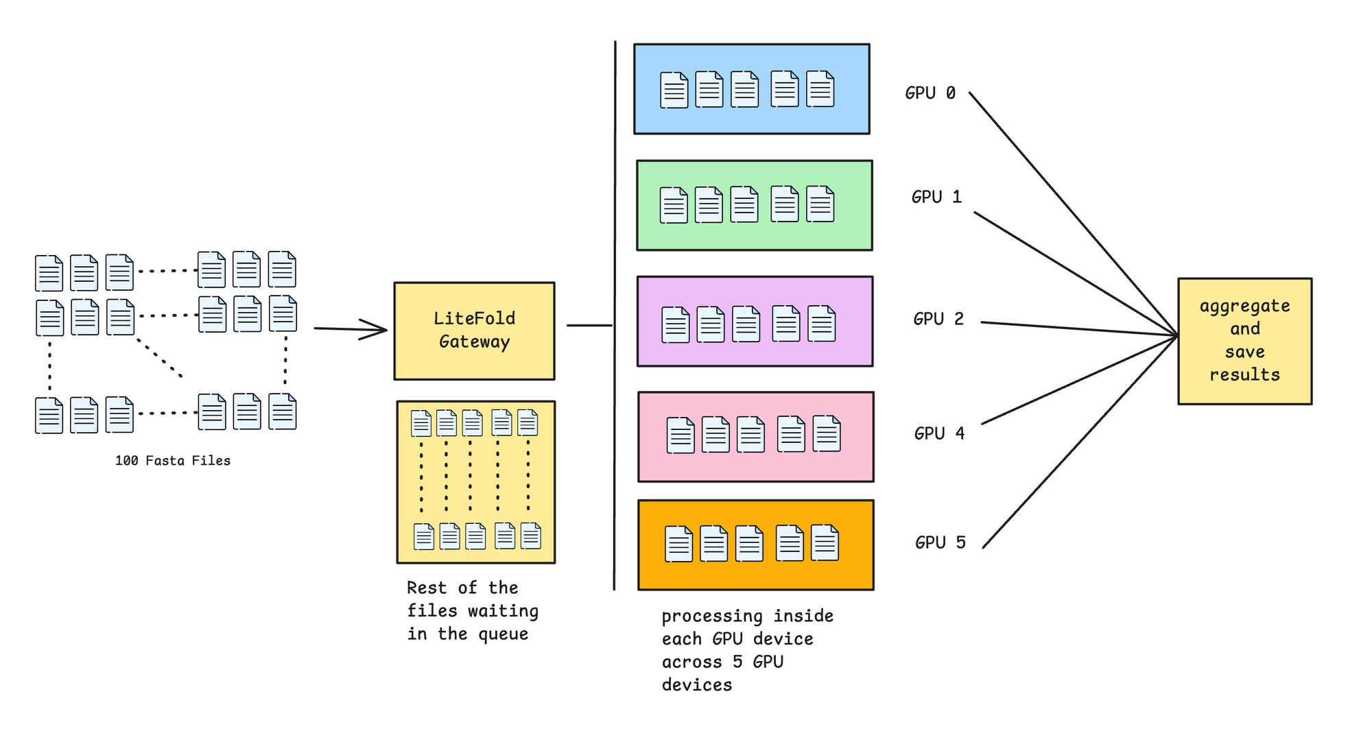
So, once you start doing structure predictions, then we handle parallelization in both ways. One is the batched inference in the same GPU. We do dynamic batching based on the residue sequence length. And accordingly, we handle batch inference. Not only that, we also handle multi GPU parallelization, where we distribute, multiple FASTA files batches in multiple GPUs. So, to put it simply, suppose you are predicting 100 fasta files. Assume, we do predictions in a batch of 5 files. So this means, we have 20 such batches. So each device (containing one GPU) will be computing 5 files and we will be having 5 gpus. So in one go we are predicting 25 FASTA files, and in just 4 passes, we will complete our overall predictions. Visually how this looks like:
Inside each GPU, we compute structure prediction, affinity prediction (if mentioned in the input to compute) and also compute different types of metrics. Metrics are super important to asses and filter the quality of the structure. Let's discuss in the next section.
Asses quality right after predictions
Once structure predictions are finished, researchers anyways tend to either write scripts or use CLIs to understand, filter and asses structure quality. However in LiteFold, we have metrics already built in. Let's discuss each of the metrics which are available in LiteFold.
Predicted Local Distance Difference Test (pLDDT)
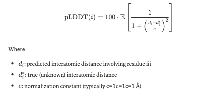
pLDDT estimates the confidence in the position of each residue in the predicted structure. It ranges from 0 to 100 (or 0 to 1 in normalized form), where higher values indicate higher confidence. For a given i, pLDDT estimates the expected distance deviation from the true structure over a small local window.
This helps visualize local model confidence per residue. Scores > 70 are generally considered trustworthy, while scores < 50 indicate low confidence. In LiteFold platform, we also color the residue structure based on the pLDDT score.
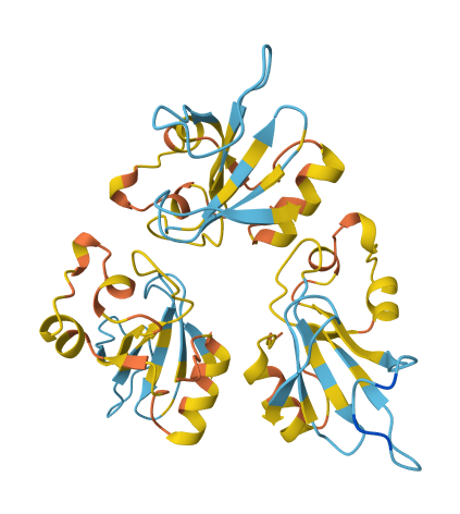
As you can see in the above picture, we have residues colored in different shades as follows:
- > 90 (dark blue): very high confidence.
- 70-90 (yellow - lightblue): confident
- < 70 (orange - red): Low confidence (might be disordered or un-certain)
These are super important, because sometimes, these folds could be associated with different binding sites / regions. So, if the confidence is not good, then the downstream follows could be subjected to change which will save a good time, because in that case you can reject the structure.
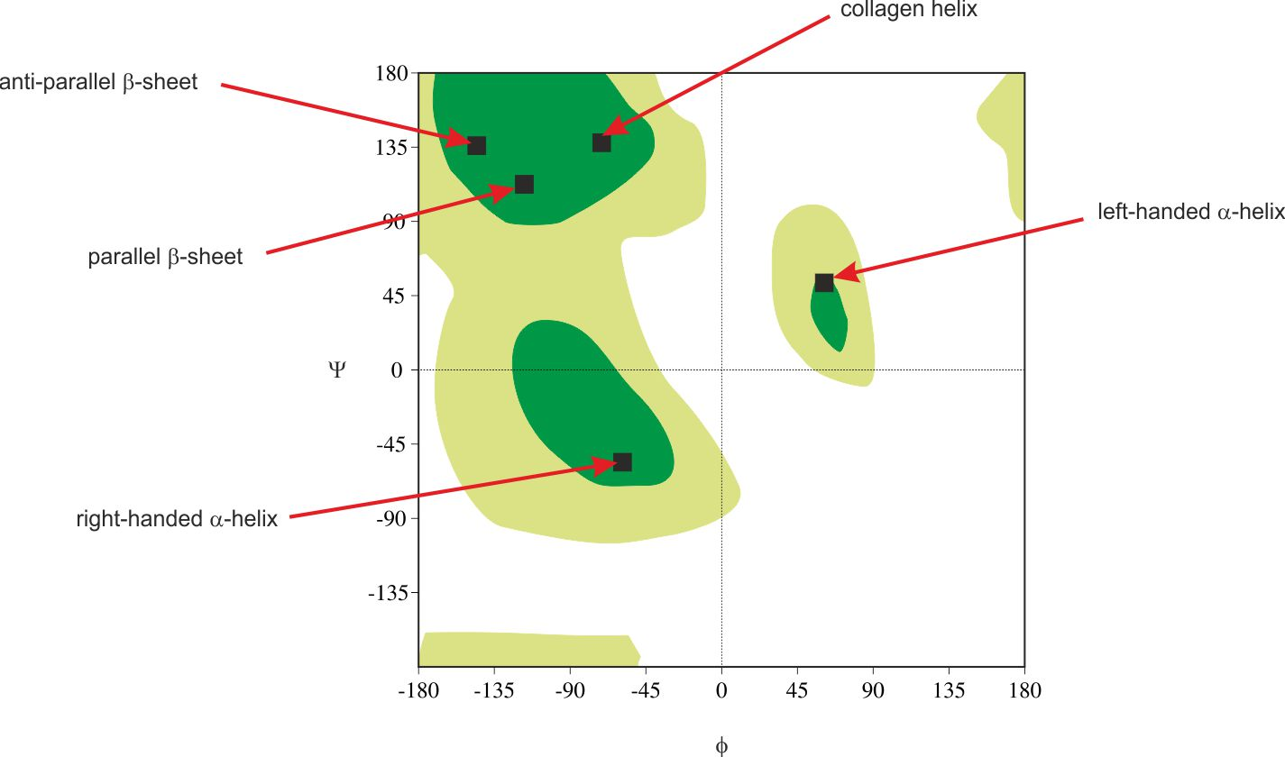
Ramachandran Plot Validation
Ramachandran plots show the distribution of backbone dihedral angles (ϕ, ψ) for residues, used to assess stereochemical quality. To put it simply, the plot helps us to visualize the allowed conformation of polypeptide backbones in the proteins. It helps to asses the quality of the protein structures and understand the preferred angles of rotations in the backbone.
Proteins are made up of amino acid and each amino acid are linked by peptide bonds. So in a polypeptide, each amino acid has a:
- A phi (ϕ) torison angle - rotation around N-Cα bond
- A psi (ψ) torsion angle - rotation around the Cα–C bond
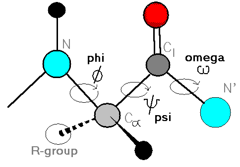
Each residue (except glycine and proline) in a protein has a specific (ϕ, ψ) combination. When you plot these, you get a map of allowed and disallowed regions based on steric hinderance.
So inside LiteFold, mathematically, for each residue ri we compute:
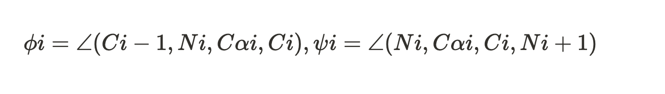
Outliers are defined as residues where (ϕi,ψi) lie outside all allowed regions. The final metric is:
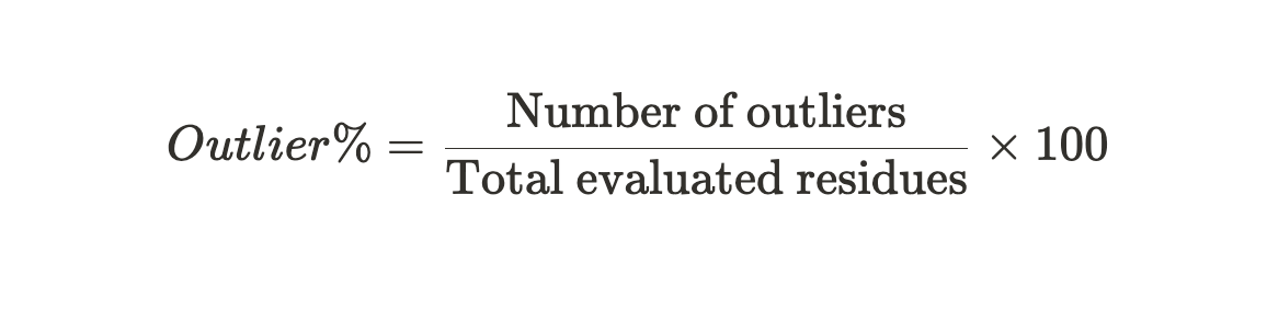
This percentage provides a quantitative measure of stereochemical quality — lower values indicate better structural geometry.
Clash Score
We compute the clash score to quantify steric overlaps (clashes) between atoms in a predicted protein structure. This follows MolProbity standards, where a clash is defined as two non-bonded atoms being closer than the sum of their van der Waals (vdW) radii minus a threshold of 0.4 Å. Small allowances are made for potential hydrogen bonds. So, let
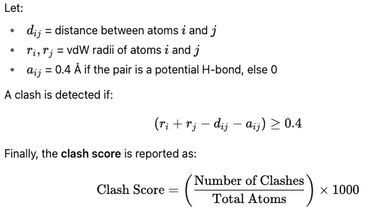
This gives the number of steric clashes per 1000 atoms — lower values indicate more physically realistic and better-packed structures.
Binding Affinity Prediction
This metric is a model based metric. This means we use another deep learning model, in our case it is Boltz-2 Affinity to predict this score. This predicts how strongly the ligand binds to the protein expressed as log(IC50) or binding probability.
The Boltz-2 Affinity model has two heads, the regression head predicts the log(IC5o [μM]), which represent the log scale inhibitory concentration (IC5o) in micromolar units. Lower values indicates stronger binding (nanomolar to picomolar) while higher values indicate weak or no binding.
The binary classifier head predicts the probability that a ligand is a binder. This is useful for hit indentification where the goal is to distinguish binders from non-binders.
So, now we can interpret binding strength in energetic terms, we can approximate Gibbs free energy of binding ΔG from the predicted log(IC₅₀) using:
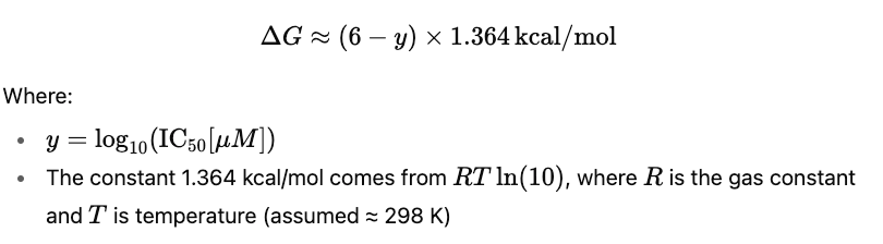
We can even compute approximate IC₅₀ and ΔG values based on the predicted log(IC₅₀) values (denoted here as y) as shown in the table below.
| Predicted | IC₅₀ (μM) | Approx. ΔG (kcal/mol) | Binding Strength |
|---|---|---|---|
| -3 | 0.001 nM | ≈12.6 | Very strong binder |
| 0 | 1 μM | ≈8.2 | Moderate binder |
| 2 | 100 μM | ≈5.5 | Weak binder / decoy |
Conclusion & What's coming next
So, that's all about LiteFold's structure prediction module. We discussed about how you can predict structures with Boltz, can edit protein residues easily, predict structures at scale. We also take a peak at different metrics, we support, what they do and their significance.
So what's coming next
In the coming versions, we will be adding support for AlphaFold-2 model as well. AlphaFold-3 might be coming later, because that requires a different integration. We will also bring more metrics so more granular filtering and evaluating structure quality.
In the end, we are making the AI-powered lab for early stage drug discovery and research. So, in the structure prediction in that respect, we will be bringing things like relaxing the structure, using molecular dynamics to see the stability of the predicted complex and many more.
However we are not just limiting ourselves to structure predictions. More sophisticated pipelines like generating denovo molecules, molecular docking, molecular dynamics are all coming soon.
Not to forget, we are also building Rosalind, our intelligent AI Co-Research assistant, which will help you to build multiple experiments faster than ever, so that you can get the results much faster and focus on doing the core research. We are super excited. Until next time.
We are on a mission to make molecular and structural biology related experiments easier than ever. Whether you are doing research on protein design, drug design or want to run and organize your experiments, LiteFold helps to manage that with ease. Do try out, it's free.